How can these 'fake' leaves help us to estimate tree transpiration?

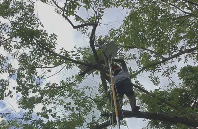
In this post, I aim to explain how leaf replicas might be used to estimate both boundary layer conductance and transpiration. Or, to put it another way, what’s the deal with those wild leaves, and why are they hanging out up in that tree?
Before giving further explanation why these replicas exists, we need to get a sense of how leaf temperature of plants is influenced by the plant itself and its environment. We can do so by looking at a leaf energy balance. That is, incoming energy mostly from the sun and emitted energy from the leaf have to be in balance to maintain a stable leaf temperature. A leaf losses energy from thermal radiation (radiation loss $S$), heat transfer to the surrounding air (sensible heat loss $C$) and a loss of water, which evaporates and cools down its surface (latent heat flux $\lambda E$), where $\lambda$ is the latent heat of evaporation, i.e., the amount energy we need to transform water into vapor.
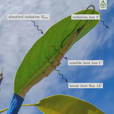
All the energy variables are summed up to form the energy balance equation, i.e., incoming energy is defined positiv and emitted (outward) energy is defined negativ.
$$ R_{abs} - S - C - \lambda E = 0 $$
Absorbed radiation
Leaf temperature increases by absorbing solar energy and infrared radiation. More sunlight, higher air temperature, and greater absorption increase energy input. The net radiation $R_n$ consists of absorbed incoming short and longwave radiation and emitted outward longwave radiation.
$$ R_n = R_{abs} - S = \underbrace{(\alpha I_s + L_d)}_{\text{incoming short + longwave}} - \overbrace{2\sigma\epsilon T^4}^{\text{outward longwave}} $$
| Parameter | Description | Units |
|---|---|---|
| $\alpha$ | Determines how much shortwave radiation can be absorbed by the leaf, can vary between 0.6 - 0.85 | - |
| $I_s$ | Incoming shortwave solar radiation (300 - 3000 $\mathrm{nm}$) up to 1000 $\mathrm{W\ m^{-2}}$ on a clear midday in Costa Rica. | $\mathrm{W\ m^{-2}}$ |
| $L_d$ | Longwave radiation (wavelengths 3 - 100 $\mathrm{\mu m}$) received from the surrounding environment (e.g., soil, other trees, sky). | $\mathrm{W\ m^{-2}}$ |
| $\sigma$ | Stefan-Boltzmann constant $5.67\mathrm{e}{-8}$ | $\mathrm{W\ m^{-2}\ K^{-4}}$ |
| $\epsilon$ | Leaf emissivity, determines how much longwave radiation is absorbed and emitted, usually between 0.96 - 0.98 | - |
| $T$ | Leaf temperature | $\mathrm{K}$ |
Sensible heat loss $C$
Leaves lose heat through convection when leaf temperature is greater than air temperature. Sensible heat flux is proportional to the temperature difference between leaf and air; more heat is lost as leaf temperature increases above air temperature.
$$ C = 2 g_{bh} \rho C_s (T - T_{air} ) $$
| Parameter | Description | Units |
|---|---|---|
| $g_{bh}$ | boundary layer conductance, depends mainly on the leaf shape and size and on the wind speed | $\mathrm{m\ s^{-1}}$ |
| $\rho$ | density of air | $\mathrm{kg\ m^{-3}}$ |
| $C_s$ | specific heat capacity of humid air | $\mathrm{J\ kg^{-1}\ K^{-1}}$ |
| $T$ | Leaf temperature | $\mathrm{K}$ |
| $T_{air}$ | Air temperature | $\mathrm{K}$ |
Now let us play around a little bit with the equation so far and calculate the transpiration rate $E$ under different environment conditions and plant parameters.
Most of the parameters needed to estimate transpiration can be measured using a weather station and an infrared thermometer to gauge leaf temperature. However, you might have noticed that boundary layer conductance plays a significant role in the energy balance and, as a result, impacts the transpiration rate. To accurately measure transpiration in the real world, we need to estimate the boundary layer conductance. This term describes the thin layer of relatively calm air surrounding a leaf, where heat transfer occurs mainly through conduction—that is, air molecules exchange energy through vibrations—rather than through convection, where air molecules are carried away by a moving air stream. One approach to estimating the boundary layer conductance is through aerodynamic theory,
$$ g_{bh} = 0.00662 \sqrt{\frac{u}{d}} $$
where $d$ represents a characteristic leaf dimension while $u$ denotes the wind velocity. For circular plates, which is a good approximation for round-shaped leaves, $d$ is taken to be 0.9 times the leaf’s diameter.
Often, wind speed data may not be available in the forested areas, particularly at the tree canopy level. Although it is sometimes possible to infer wind speeds at different heights using ground-level measurements, the actual wind speeds within the forest or even within the canopy might be different and are effected by turbulence.
Alternatively, we can use the energy balance equation to solve for $g_{bh}$. However, to do so we need to know the transpiration $E$. This is where we take our ‘fake’ leaves, they do not transpire but have a similar shape to the real leaves and are exposed to the exact same environment within the canopy. So let us set $E = 0$ and solve for $g_{bh}$. We can extend this idea of parameter elimination even further: by using two replica leaves, we can avoid estimating the longwave incoming radiation. Let’s write down the energy balance for two non-transpiring leaf replicas, one white ($T_w$) and one black ($T_b$):
$$\alpha_{w}I_s + L_d - 2\sigma\epsilon_{w} T_{w}^4 - 2 g_{bh}\rho C_s (T_{w} - T_{air}) = k \frac{dT_{w}}{dt} $$ $$\alpha_{b}I_s + L_d - 2\sigma\epsilon_{b} T_{b}^4 - 2 g_{bh}\rho C_s (T_{b} - T_{air}) = k \frac{dT_{b}}{dt} $$
Note that the we must not set the energy balance to zero as before, if the energy balance is not zero the remaining energy will heat up or cool down the leaf. We express this change in temperature over time as $k \frac{dT}{dt} $, where $k$ is the amount of energy per area required to change the temperature of the leaf by 1 $\mathrm{K}$ or 1°C expressed in $\mathrm{J\ m^{-2}\ K^{-1}}$. We combine both equations by subtracting them and solve for $g_{bh}$:
$$ g_{bh} = \frac{k(\frac{dT_w}{dt} - \frac{dT_b}{dt}) - I_s(\alpha_w - \alpha_b) + 2\sigma(\epsilon_w T_w^4 - \epsilon_b T_b^4)}{2\rho C_s (T_b - T_w)} $$
If both leaf replicas absorb the same amount of longwave radiation, i.e., they have similar emissivity $(\epsilon_w \approx \epsilon_b)$, we do not need to consider long wave radiation 😎.
Let us calculate the boundary layer conductance for some data from Costa Rica recorded on the 2022-02-26 at 12:00:
The black painted replica reached temperatures up to 56 °C, while the white replica was on average 15 °C colder. Fluctuation in temperature are caused by wind gust, which reached up to $7.3\ \mathrm{m\ s^{-1}}$. Temperature was recorded every 10 s with a digital temperature sensor (Dallas DS1820) attached to the replica leaf. Data points were interpolate by a spline and the spline derivative was used to calculate $\frac{dT}{dt}$. Other parameters needed to calculate the boundary layer conductance are given below.
| Parameter | Description | Value |
|---|---|---|
| $k = l \rho c_p$ | Replica leaf thickness $l = 0.45\ \mathrm{mm}$, density of leaf replica (galvanized steel) $\rho = 7850\ \mathrm{kg\ m^{-3}}$ and specific heat capacity of steel $ c_p = 420\ \mathrm{J\ kg^{-1}\ K^{-1}}$ | $1484\ \mathrm{J\ m^{-2}\ K^{-1}}$ |
| $I_s$ | Incoming shortwave radiation | $900\ \mathrm{W\ m^{-2}}$ |
| $\alpha_w, \alpha_b$ | Shortwave radiation absorption coefficient for the white and black replica, the black paint will absorb a lot more sun light compared to the white one | 0.1, 0.9 |
| $\epsilon_w, \epsilon_b$ | Emissivity of the white and black replica | 0.95, 0.95 |
| $\rho$ | Density of air, we assume dry air at standard atmospheric pressure | $1.225\ \mathrm{kg\ m^{-3}}$ |
| $C_s$ | Specific heat capacity of air, we assume dry air again. Air at room temperature with 100% relative humidity will have a slightly higher heat capacity of $1184\ \mathrm{J\ kg^{-1}\ K^{-1}}$ | $1005\ \mathrm{J\ kg^{-1}\ K^{-1}}$ |
Resulting boundary layer conductance:
We can see that the boundary layer conductance is not constant, we would expect similar results if we use the aerodynamic theory as the boundary layer conductance is affected by wind. On average conductance fluctuates around $16\ \mathrm{mm\ s^{-1}}$ but reaches values up to $40\ \mathrm{mm\ s^{-1}}$. Given our estimate of $g_{bh}$, we can calculate the transpiration rate for a real leaf. Leaf temperature was measure every 10 s by a PT100 thermistor attached to the downside of a leaf (maybe you already noticed, if not the leaf sensor can be seen in leaf energy budget figure 🧐).
To do so, we now consider one “fake leaf” ($T_w$) and a real leaf ($T_l$):
$$\alpha_{w}I_s + L_d - 2\sigma\epsilon_{w} T_{w}^4 - 2 g_{bh}\rho C_s (T_{w} - T_{air}) = k \frac{dT_{w}}{dt} $$ $$\alpha_{l}I_s + L_d - 2\sigma\epsilon_{l} T_{l}^4 - 2 g_{bh}\rho C_s (T_{l} - T_{air}) - \lambda E = k_l \frac{dT_{l}}{dt} $$
and again we combine both equations by subtracting them, however this time we solve for $\lambda E$ to estimate the transpiration:
$$\lambda E = k \frac{dT_{w}}{dt} - k_l \frac{dT_{l}}{dt} - (\alpha_w - \alpha_l)I_s$$ $$ - 2\sigma(\epsilon_l T_{l}^4 - \epsilon_w T_{w}^4) - 2 g_{bh}\rho C_s (T_l - T_w)$$
| Parameter | Description | Value |
|---|---|---|
| $k_l = l \rho c_p$ | Real leaf thickness $l = 0.3\ \mathrm{mm}$, density of real leaf $\rho = 750\ \mathrm{kg\ m^{-3}}$ and specific heat capacity of real leaf $ c_p = 3000\ \mathrm{J\ kg^{-1}\ K^{-1}}$ | $675\ \mathrm{J\ m^{-2}\ K^{-1}}$ |
| $\alpha_l$ | Shortwave radiation absorption coefficient of a real leaf | 0.5 |
| $\epsilon_l$ | Emissivity of a real leaf | 0.95 |
Resulting transpiration rate from the energy balance model:
Again we see a lot of fluctuations caused by the changes in leaf temperature. On average we estimate a transpiration rate of $8\ \mathrm{mmol\ m^{-2}\ s^{-1}}$, this would mean that a leaf area of 1 m² would release around 0.5 liter of water in one hour 😲.
I hope you learned something :) and understood how ‘fake’ leaves potentially can be used to estimate the boundary layer conductance and transpiration. Now, none of the calculations were validated so the results should be taken with caution, more work to be done as always 😄.
The takeaway for me would be that, we should be careful when we analyze thermal images as they might only be a snapshot of a constantly changing environment or in our case changing leaf temperature. Ideally, images would be taken in a complete stable environment but often this is not the case. By continuously recording leaf replica temperatures we get a quick check how stable our environment is and hopefully we can use that information to get more reliable transpiration data even in changing conditions.
References
Jones, Hamlyn G. Plants and Microclimate: A Quantitative Approach to Environmental Plant Physiology. Cambridge university press, 2013.
Vialet-Chabrand, Silvere, and Tracy Lawson. “Dynamic Leaf Energy Balance: Deriving Stomatal Conductance from Thermal Imaging in a Dynamic Environment.” Journal of Experimental Botany 70, no. 10 (2019): 2839–55.
Vialet-Chabrand, Silvere, and Tracy Lawson. “Thermography Methods to Assess Stomatal Behaviour in a Dynamic Environment.” Journal of Experimental Botany 71, no. 7 (2020): 2329–38.